Optimization Algorithms: Overview
1. The basics
1.1. Search space size in the real world
The number of possible solutions for a planning problem can be mind blowing. For example:
-
Four queens has
256possible solutions (4^4) and two optimal solutions. -
Five queens has
3125possible solutions (5^5) and one optimal solution. -
Eight queens has
16777216possible solutions (8^8) and 92 optimal solutions. -
64 queens has more than
10^115possible solutions (64^64). -
Most real-life planning problems have an incredible number of possible solutions and only one or a few optimal solutions.
For comparison: the minimal number of atoms in the known universe (10^80). As a planning problem gets bigger, the search space tends to blow up really fast. Adding only one extra planning entity or planning value can heavily multiply the running time of some algorithms. Calculating the number of possible solutions depends on the design of the domain model:
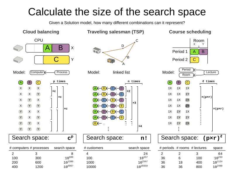
|
This search space size calculation includes infeasible solutions (if they can be represented by the model), because:
Even in cases where adding some of the hard constraints in the formula is practical, the resulting search space is still huge. |
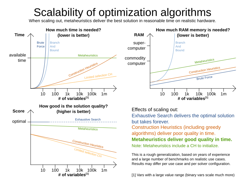
An algorithm that checks every possible solution (even with pruning, such as in Branch And Bound) can easily run for billions of years on a single real-life planning problem. The aim is to find the best solution in the available timeframe. Planning competitions (such as the International Timetabling Competition) show that Local Search usually performs best for real-world problems given real-world time limitations.
1.2. Does Timefold Solver find the optimal solution?
The business wants the optimal solution, but they also have other requirements:
-
Scale out: Large production data sets must not crash and have also good results.
-
Optimize the right problem: The constraints must match the actual business needs.
-
Available time: The solution must be found in time, before it becomes useless to execute.
-
Reliability: Every data set must have at least a decent result (better than a human planner).
Given these requirements, and despite the promises of some salesmen, it is usually impossible for anyone or anything to find the optimal solution. Therefore, Timefold Solver focuses on finding the best solution in available time.
The nature of NP-complete problems make scaling a prime concern.
|
The quality of a result from a small data set is no indication of the quality of a result from a large data set. |
Scaling issues cannot be mitigated by hardware purchases later on. Start testing with a production sized data set as soon as possible. Do not assess quality on small data sets (unless production encounters only such data sets). Instead, solve a production sized data set and compare the results of longer executions, different algorithms and - if available - the human planner.
1.3. Supported optimization algorithms
Timefold Solver supports three families of optimization algorithms: Exhaustive Search, Construction Heuristics and Metaheuristics. In practice, Metaheuristics (in combination with Construction Heuristics to initialize) are the recommended choice:
Each of these algorithm families have multiple optimization algorithms:
| Algorithm | Scalable? | Optimal? | Easy to use? | Tweakable? | Requires CH? |
|---|---|---|---|---|---|
Exhaustive Search (ES) |
|||||
0/5 |
5/5 |
5/5 |
0/5 |
No |
|
0/5 |
5/5 |
4/5 |
2/5 |
No |
|
5/5 |
1/5 |
5/5 |
1/5 |
No |
|
5/5 |
2/5 |
4/5 |
2/5 |
No |
|
5/5 |
2/5 |
4/5 |
2/5 |
No |
|
5/5 |
2/5 |
4/5 |
2/5 |
No |
|
5/5 |
2/5 |
4/5 |
2/5 |
No |
|
5/5 |
2/5 |
4/5 |
2/5 |
No |
|
3/5 |
2/5 |
5/5 |
2/5 |
No |
|
3/5 |
2/5 |
5/5 |
2/5 |
No |
|
Metaheuristics (MH) |
|||||
Local Search (LS) |
|||||
5/5 |
2/5 |
4/5 |
3/5 |
Yes |
|
5/5 |
4/5 |
3/5 |
5/5 |
Yes |
|
5/5 |
4/5 |
2/5 |
5/5 |
Yes |
|
5/5 |
4/5 |
3/5 |
5/5 |
Yes |
|
5/5 |
4/5 |
3/5 |
5/5 |
Yes |
|
5/5 |
4/5 |
3/5 |
5/5 |
Yes |
|
3/5 |
3/5 |
2/5 |
5/5 |
Yes |
|
To learn more about metaheuristics, see Essentials of Metaheuristics or Clever Algorithms.
1.4. Which optimization algorithms should I use?
The best optimization algorithm configuration to use depends heavily on your use case. However, this basic procedure provides a good starting configuration that will produce better than average results.
-
Start with a quick configuration that involves little or no configuration and optimization code: See First Fit.
-
Next, implement planning entity sorting and turn it into First Fit Decreasing.
-
Next, add Late Acceptance behind it:
-
First Fit Decreasing.
-
At this point, the return on invested time lowers and the result is likely to be sufficient.
However, this can be improved at a lower return on invested time. Use the Benchmarker and try a couple of different Tabu Search, Simulated Annealing and Late Acceptance configurations, for example:
-
First Fit Decreasing
Use the Benchmarker to improve the values for the size parameters.
Other experiments can also be run. For example, the following multiple algorithms can be combined together:
-
First Fit Decreasing
-
Late Acceptance (relatively long time)
-
Tabu Search (relatively short time)
2. Architecture
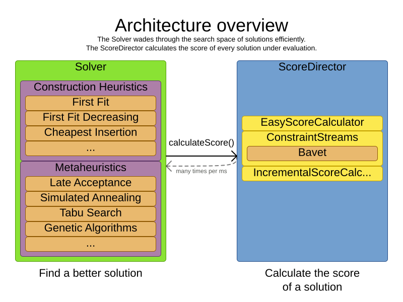
Timefold Solver combines optimization algorithms (metaheuristics, …) with score calculation by a score calculation engine. This combination is very efficient, because:
-
A score calculation engine is great for calculating the score of a solution of a planning problem. It makes it easy and scalable to add additional soft or hard constraints. It does incremental score calculation (deltas) without any extra code. However it tends to be not suitable to actually find new solutions.
-
An optimization algorithm is great at finding new improving solutions for a planning problem, without necessarily brute-forcing every possibility. However, it needs to know the score of a solution and offers no support in calculating that score efficiently.
2.1. Power tweaking or default parameter values
Many optimization algorithms have parameters that affect results and scalability. Timefold Solver applies configuration by exception, so all optimization algorithms have default parameter values. This is very similar to the Garbage Collection parameters in a JVM: most users have no need to tweak them, but power users often do.
The default parameter values are sufficient for many cases (and especially for prototypes), but if development time allows, it may be beneficial to power tweak them with the benchmarker for better results and scalability on a specific use case. The documentation for each optimization algorithm also declares the advanced configuration for power tweaking.
|
The default value of parameters will change between minor versions, to improve them for most users. The advanced configuration can be used to prevent unwanted changes, however, this is not recommended. |
2.2. Solver phase
A Solver can use multiple optimization algorithms in sequence.
Each optimization algorithm is represented by one solver Phase.
There is never more than one Phase solving at the same time.
|
Some |
Here is a configuration that runs three phases in sequence:
<solver xmlns="https://timefold.ai/xsd/solver" xmlns:xsi="http://www.w3.org/2001/XMLSchema-instance"
    xsi:schemaLocation="https://timefold.ai/xsd/solver https://timefold.ai/xsd/solver/solver.xsd">
  ...
  <constructionHeuristic>
    ... <!-- First phase: First Fit Decreasing -->
  </constructionHeuristic>
  <localSearch>
    ... <!-- Second phase: Late Acceptance -->
  </localSearch>
  <localSearch>
    ... <!-- Third phase: Tabu Search -->
  </localSearch>
</solver>
The solver phases are run in the order defined by solver configuration.
-
When the first
Phaseterminates, the secondPhasestarts, and so on. -
When the last
Phaseterminates, theSolverterminates.
Usually, a Solver will first run a construction heuristic and then run one or multiple metaheuristics:
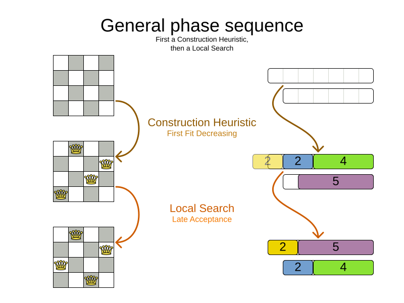
If no phases are configured, Timefold Solver will default to a Construction Heuristic phase followed by a Local Search phase.
Some phases (especially construction heuristics) will terminate automatically.
Other phases (especially metaheuristics) will only terminate if the Phase is configured to terminate:
<solver xmlns="https://timefold.ai/xsd/solver" xmlns:xsi="http://www.w3.org/2001/XMLSchema-instance"
    xsi:schemaLocation="https://timefold.ai/xsd/solver https://timefold.ai/xsd/solver/solver.xsd">
  ...
  <termination><!-- Solver termination -->
    <secondsSpentLimit>90</secondsSpentLimit>
  </termination>
  <localSearch>
    <termination><!-- Phase termination -->
      <secondsSpentLimit>60</secondsSpentLimit><!-- Give the next phase a chance to run too, before the Solver terminates -->
    </termination>
    ...
  </localSearch>
  <localSearch>
    ...
  </localSearch>
</solver>
If the Solver terminates (before the last Phase terminates itself),
the current phase is terminated and all subsequent phases will not run.
2.3. Scope overview
A solver will iteratively run phases. Each phase will usually iteratively run steps. Each step, in turn, usually iteratively runs moves. These form four nested scopes:
-
Solver
-
Phase
-
Step
-
Move

Configure logging to display the log messages of each scope.
2.4. Termination
Not all phases terminate automatically and may take a significant amount of time.
A Solver can be terminated synchronously by up-front configuration, or asynchronously from another thread.
Metaheuristic phases in particular need to be instructed to stop solving. This can be because of a number of reasons, for example, if the time is up, or the perfect score has been reached just before its solution is used. Finding the optimal solution cannot be relied on (unless you know the optimal score), because a metaheuristic algorithm is generally unaware of the optimal solution.
This is not an issue for real-life problems, as finding the optimal solution may take more time than is available. Finding the best solution in the available time is the most important outcome.
|
If no termination is configured (and a metaheuristic algorithm is used),
the |
For synchronous termination, configure a Termination on a Solver or a Phase when it needs to stop.
Every Termination can calculate a time gradient (needed for some optimization algorithms),
which is a ratio between the time already spent solving and the estimated entire solving time of the Solver or Phase.
2.4.1. Choosing the right termination
There are several aspects to consider when choosing a termination, such as the problem size, the hardware used, and the desired quality of the solution. In general:
-
Time-based terminations (such as unimproved time spent) are hardware-specific. Running the solver for 5 minutes on a laptop will yield very different results, compared to running the same solver for the same 5 minutes on a supercomputer.
-
Counting terminations (such as step count) are useful for debugging, but in the real world they do not scale well with the problem size. The solver will need many more steps to solve a large problem than it needs to solve a small problem.
-
Score-based terminations (such as best score) assume you know the target score ahead of time, which is typically not the case. And even when you do, this score is dependent on the dataset and on the constraint weights configured.
For the best experience overall, we recommend using the Diminished Returns termination. It is based on the rate of improvement of the solver, and should therefore be mostly independent of the factors listed above.
2.4.2. Combining multiple terminations
Terminations can be combined. The following example will terminate the solver when the rate of improvement drops off or after the solver has already run for 5 minutes, whichever comes first:
  <termination>
    <terminationCompositionStyle>OR</terminationCompositionStyle>
    <diminishedReturns />
    <minutesSpentLimit>5</minutesSpentLimit>
  </termination>
Alternatively you can use AND.
The following example will terminate after reaching a feasible score of at least -100 and no improvements in 5 steps:
  <termination>
    <terminationCompositionStyle>AND</terminationCompositionStyle>
    <bestScoreLimit>-100</bestScoreLimit>
    <unimprovedStepCountLimit>5</unimprovedStepCountLimit>
  </termination>
This example ensures it does not just terminate after finding a feasible solution, but also completes any obvious improvements on that solution before terminating.
2.4.3. Asynchronous termination from another thread
Asynchronous termination cannot be configured by a Termination as it is impossible to predict when and if it will occur.
For example, a user action or a server restart could require a solver to terminate earlier than predicted.
To terminate a solver from another thread asynchronously
call the terminateEarly() method from another thread:
-
Java
solver.terminateEarly();The solver then terminates at its earliest convenience.
After termination,
the Solver.solve(Solution) method returns in the solver thread (which is the original thread that called it).
|
When an To guarantee a graceful shutdown of a thread pool that contains solver threads,
an interrupt of a solver thread has the same effect as calling |
2.4.4. Available terminations
Time spent termination
Terminates when an amount of time has been used.
  <termination>
    <!-- 2 minutes and 30 seconds in ISO 8601 format P[n]Y[n]M[n]DT[n]H[n]M[n]S -->
    <spentLimit>PT2M30S</spentLimit>
  </termination>
Alternatively to a java.util.Duration in ISO 8601 format, you can also use:
-
Milliseconds
<termination> <millisecondsSpentLimit>500</millisecondsSpentLimit> </termination> -
Seconds
<termination> <secondsSpentLimit>10</secondsSpentLimit> </termination> -
Minutes
<termination> <minutesSpentLimit>5</minutesSpentLimit> </termination> -
Hours
<termination> <hoursSpentLimit>1</hoursSpentLimit> </termination> -
Days
  <termination>
    <daysSpentLimit>2</daysSpentLimit>
  </termination>
Multiple time types can be used together, for example to configure 150 minutes, either configure it directly:
  <termination>
    <minutesSpentLimit>150</minutesSpentLimit>
  </termination>
Or use a combination that sums up to 150 minutes:
  <termination>
    <hoursSpentLimit>2</hoursSpentLimit>
    <minutesSpentLimit>30</minutesSpentLimit>
</termination>|
This
|
Unimproved time spent termination
Terminates when the best score has not improved in a specified amount of time. Each time a new best solution is found, the timer basically resets.
  <localSearch>
    <termination>
      <!-- 2 minutes and 30 seconds in ISO 8601 format P[n]Y[n]M[n]DT[n]H[n]M[n]S -->
      <unimprovedSpentLimit>PT2M30S</unimprovedSpentLimit>
    </termination>
  </localSearch>
Alternatively to a java.util.Duration in ISO 8601 format, you can also use:
-
Milliseconds
<localSearch> <termination> <unimprovedMillisecondsSpentLimit>500</unimprovedMillisecondsSpentLimit> </termination> </localSearch> -
Seconds
<localSearch> <termination> <unimprovedSecondsSpentLimit>10</unimprovedSecondsSpentLimit> </termination> </localSearch> -
Minutes
<localSearch> <termination> <unimprovedMinutesSpentLimit>5</unimprovedMinutesSpentLimit> </termination> </localSearch> -
Hours
<localSearch> <termination> <unimprovedHoursSpentLimit>1</unimprovedHoursSpentLimit> </termination> </localSearch> -
Days
  <localSearch>
    <termination>
      <unimprovedDaysSpentLimit>1</unimprovedDaysSpentLimit>
    </termination>
  </localSearch>
Just like time spent termination, combinations are summed up.
It is preffered to configure this termination on a specific Phase (such as <localSearch>) instead of on the Solver itself.
Several phases, such as construction heuristics, do not count towards this termination because they only trigger new best solution events when they are done. If such a phase is encountered, the termination is disabled and when the next phase is started, the termination is enabled again and the timer resets back to zero. In the most typical case, where a local search phase follows a construction heuristic phase, the termination will only trigger if the local search phase does not improve the best solution for the specified time.
|
This
|
Optionally, configure a score difference threshold by which the best score must improve in the specified time.
For example, if the score doesn’t improve by at least 100 soft points every 30 seconds or less, it terminates:
  <localSearch>
    <termination>
      <unimprovedSecondsSpentLimit>30</unimprovedSecondsSpentLimit>
      <unimprovedScoreDifferenceThreshold>0hard/100soft</unimprovedScoreDifferenceThreshold>
    </termination>
  </localSearch>
If the score improves by 1 hard point and drops 900 soft points, it’s still meets the threshold,
because 1hard/-900soft is larger than the threshold 0hard/100soft.
On the other hand, a threshold of 1hard/0soft is not met by any new best solution
that improves 1 hard point at the expense of 1 or more soft points,
because 1hard/-100soft is smaller than the threshold 1hard/0soft.
To require a feasibility improvement every 30 seconds while avoiding the pitfall above,
use a wildcard * for lower score levels that are allowed to deteriorate if a higher score level improves:
  <localSearch>
    <termination>
      <unimprovedSecondsSpentLimit>30</unimprovedSecondsSpentLimit>
      <unimprovedScoreDifferenceThreshold>1hard/*soft</unimprovedScoreDifferenceThreshold>
    </termination>
  </localSearch>
This effectively implies a threshold of 1hard/-2147483648soft, because it relies on Integer.MIN_VALUE.
BestScoreTermination
BestScoreTermination terminates when a certain score has been reached.
Use this Termination where the perfect score is known,
for example for four queens (which uses a SimpleScore):
  <termination>
    <bestScoreLimit>0</bestScoreLimit>
  </termination>
A planning problem with a HardSoftScore may look like this:
  <termination>
    <bestScoreLimit>0hard/-5000soft</bestScoreLimit>
  </termination>
A planning problem with a BendableScore with three hard levels and one soft level may look like this:
  <termination>
    <bestScoreLimit>[0/0/0]hard/[-5000]soft</bestScoreLimit>
  </termination>
In this instance, Termination once a feasible solution has been reached is not practical because it requires a bestScoreLimit such as 0hard/-2147483648soft. Use the next termination instead.
BestScoreFeasibleTermination
Terminates as soon as a feasible solution has been discovered.
  <termination>
    <bestScoreFeasible>true</bestScoreFeasible>
  </termination>
This Termination is usually combined with other terminations.
StepCountTermination
Terminates when a number of steps has been reached. This is useful for hardware performance independent runs.
  <localSearch>
    <termination>
      <stepCountLimit>100</stepCountLimit>
    </termination>
  </localSearch>
This Termination can only be used for a Phase (such as <localSearch>), not for the Solver itself.
UnimprovedStepCountTermination
Terminates when the best score has not improved in a number of steps. This is useful for hardware performance independent runs.
  <localSearch>
    <termination>
      <unimprovedStepCountLimit>100</unimprovedStepCountLimit>
    </termination>
  </localSearch>
If the score has not improved recently, it is unlikely to improve in a reasonable timeframe. It has been observed that once a new best solution is found (even after a long time without improvement on the best solution), the next few steps tend to improve the best solution.
This Termination can only be used for a Phase (such as <localSearch>), not for the Solver itself.
ScoreCalculationCountTermination
ScoreCalculationCountTermination terminates when a number of score calculations have been reached.
This is often the sum of the number of moves and the number of steps.
This is useful for benchmarking.
  <termination>
    <scoreCalculationCountLimit>100000</scoreCalculationCountLimit>
  </termination>
Switching EnvironmentMode can heavily impact when this termination ends.
MoveCountTermination
MoveCountTermination terminates when a number of evaluated moves have been reached.
This is useful for benchmarking.
  <termination>
    <moveCountLimit>100000</moveCountLimit>
  </termination>
Switching EnvironmentMode can heavily impact when this termination ends.
DiminishedReturnsTermination
To save on CPU costs, you might want to terminate the solver early if expected improvements are minimal. This is hard to configure with absolute terminations since:
-
For time-based absolute terminations, they depend on the hardware used for solving. A computer that is twice as powerful should be given half the time.
-
For score-based absolute terminations, they depend on the problem. A problem with many entities will have larger score improvements than a problem with few entities.
For these situations, the diminished returns termination is desirable since it terminates based on the relative rate of improvement, and behaves similarly on different hardware and different problem instances.
The diminished returns termination terminates when the rate of improvement is below a percentage of the initial rate of improvement. The rate of improvement is the softest score difference between the final best score and the initial best score in a window, divided by the duration of the window. The first window is called a grace period, which cannot trigger a termination. If the hard score improves, the grace period is reset and the initial rate of improvement is recalculated.
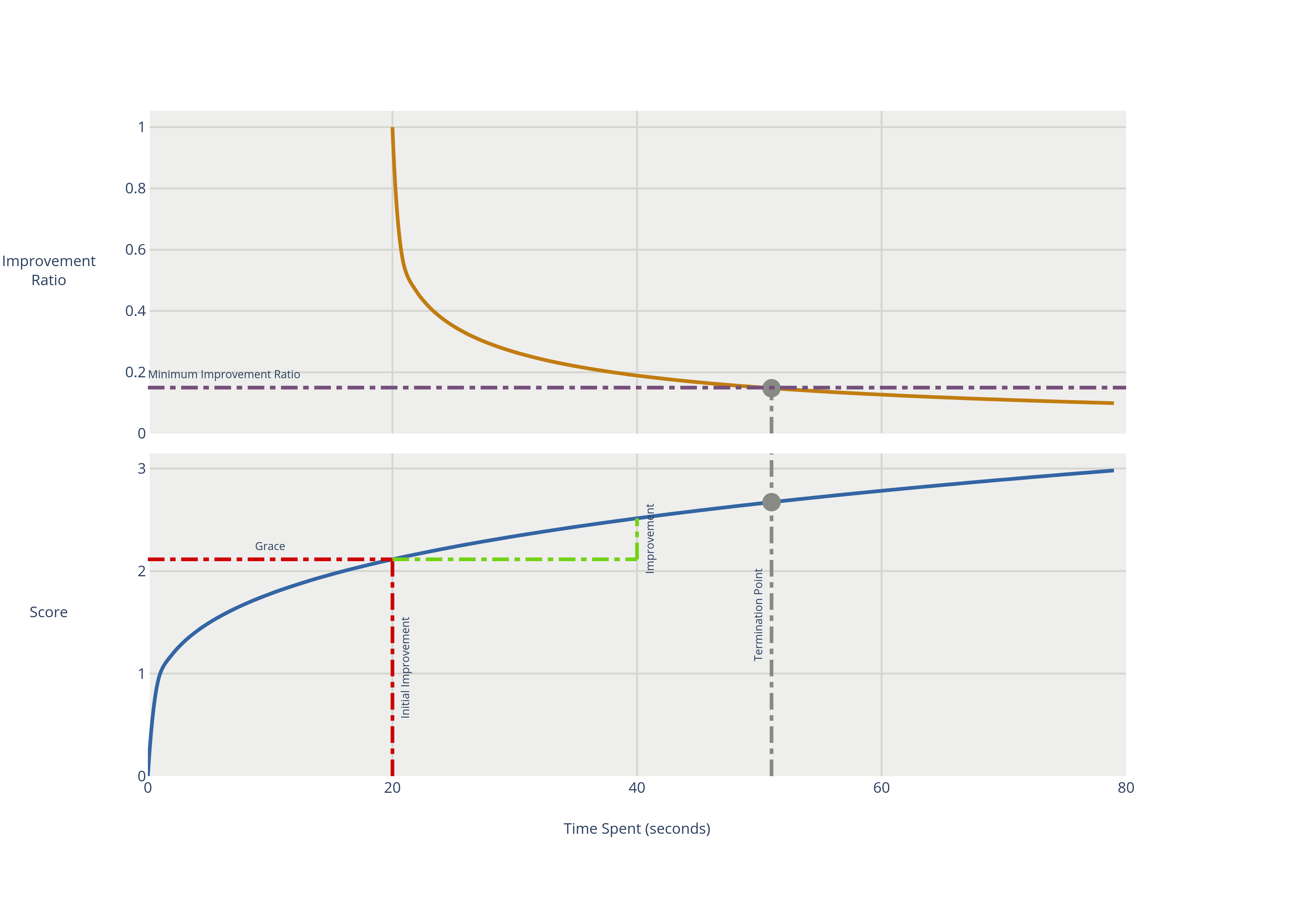
  <localSearch>
    <termination>
      <diminishedReturns />
    </termination>
  </localSearch>
There are two properties that can optionally be configured:
-
slidingWindowDuration, which is the initial grace period and is the length of the window that is used for the rate of improvement calculation.<localSearch> <termination> <diminishedReturns> <slidingWindowDuration>PT2M30S</slidingWindowDuration> </diminishedReturns> </termination> </localSearch>Alternatively to a
java.util.Durationin ISO 8601 format, you can also use milliseconds, seconds, minutes, hours or days:<localSearch> <termination> <diminishedReturns> <slidingWindowSeconds>500</slidingWindowSeconds> </diminishedReturns> </termination> </localSearch> -
minimumImprovementRatio, which is the minimum value that the ratio between the current and the initial rate of change can be to prevent termination. For instance, ifminimumImprovementRatiois0.2, then the current rate of change must be20%of the initial rate of change to prevent termination.<localSearch> <termination> <diminishedReturns> <minimumImprovementRatio>0.2</minimumImprovementRatio> </diminishedReturns> </termination> </localSearch>
2.5. SolverEventListener
Each time a new best solution is found, a new BestSolutionChangedEvent is fired in the Solver thread.
To listen to such events, add a SolverEventListener to the Solver:
-
Java
public interface Solver<Solution_> {
    ...

    void addEventListener(SolverEventListener<S> eventListener);
    void removeEventListener(SolverEventListener<S> eventListener);

}
The BestSolutionChangedEvent's newBestSolution may not be initialized or feasible.
Use the isFeasible() method on BestSolutionChangedEvent's new best Score to detect such cases.
Use the event’s isNewBestSolutionInitialized() method to only ignore uninitialized solutions,
but also accept infeasible solutions.
|
The |
2.6. Custom solver phase
Run a custom optimization algorithm between phases or before the first phase to initialize the solution, or to get a better score quickly.
You will still want to reuse the score calculation.
For example, to implement a custom Construction Heuristic without implementing an entire Phase.
|
Most of the time, a custom solver phase is not worth the investment of development time. Construction Heuristics are configurable and support partially initialized solutions too. You can use the Benchmarker to tweak them. |
The PhaseCommand interface appears as follows:
public interface PhaseCommand<Solution_> {

    void changeWorkingSolution(PhaseCommandContext<Solution_> commandContext);

}
The PhaseCommandContext interface offers the following methods:
Object getWorkingSolution()-
Returns the working solution of the
Solverthat is being solved. This must not be directly modified, as that would corrupt theSolver. void execute(Move)-
Executes a
Moveon the working solution. This is the only way to change the working solution without corrupting theSolver. Users can either provide a customMoveimplementation, or choose from theMoveimplementations provided out-of-the-box.getSolutionMetaModel()method ofPhaseCommandContextcan be used to get theSolutionMetaModelof the working solution, which will help with creating theseMoveinstances. Object executeTemporarily(Move, Function)-
As defined above, but the executed move is immediately undone. The provided
Functionis executed while the move is still applied, so that the user can perform arbitrary calculations on the working solution with the move applied. The return value of the providedFunctionis returned by this method. boolean isPhaseTerminated()-
Returns
trueif thePhaseCommandshould terminate. Object lookupWorkingObject(Object externalObject)-
Returns the working object that corresponds to the given external object. This is useful when the
PhaseCommandremembers an object from some previous working solution, and needs to find the corresponding object in the current working solution, which may have been planning-cloned since.
Any change on the planning entities in a PhaseCommand must be done through the execute(Move) method,
to avoid corrupting the Solver.
Long-running commands may want to periodically check isPhaseTerminated and when it returns true,
terminate the command by returning.
The solver will only terminate after the command returns.
|
Do not change any of the problem facts in a |
Configure the PhaseCommand in the solver configuration:
<solver xmlns="https://timefold.ai/xsd/solver" xmlns:xsi="http://www.w3.org/2001/XMLSchema-instance"
    xsi:schemaLocation="https://timefold.ai/xsd/solver https://timefold.ai/xsd/solver/solver.xsd">
  ...
  <customPhase>
    <customPhaseCommandClass>...MyCustomPhase</customPhaseCommandClass>
  </customPhase>
  ... <!-- Other phases -->
</solver>
Configure multiple customPhaseCommandClass instances to run them in sequence.
|
If the changes performed in a |
To configure values of a PhaseCommand dynamically in the solver configuration
(so the Benchmarker can tweak those parameters),
add the customProperties element and use custom properties:
  <customPhase>
    <customPhaseCommandClass>...MyCustomPhase</customPhaseCommandClass>
    <customProperties>
      <property name="mySelectionSize" value="5"/>
    </customProperties>
  </customPhase>
3. Move and neighborhood selection
3.1. What is a Move?
A Move is a change (or set of changes) from a solution A to a solution B.
For example, the move below changes queen C from row 0 to row 2:
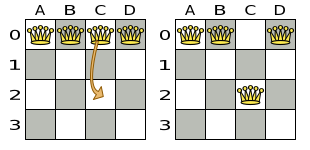
The new solution is called a neighbor of the original solution, because it can be reached in a single Move.
Although a single move can change multiple queens,
the neighbors of a solution should always be a tiny subset of all possible solutions.
For example, on that original solution, these are all possible changeMoves:
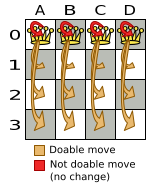
If we ignore the four changeMoves that have no impact and are therefore not doable, we can see that the number of moves is n * (n - 1) = 12.
This is far less than the number of possible solutions, which is n ^ n = 256.
As the problem scales out, the number of possible moves increases far less than the number of possible solutions.
Yet, in four changeMoves or less we can reach any solution.
For example we can reach a very different solution in three changeMoves:
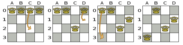
There are many other types of moves besides changeMoves.
Many move types are included out-of-the-box, but you can also implement custom moves.
A Move can affect multiple entities, but it must not change the problem facts,
add or remove entities.
|
All optimization algorithms use Moves to transition from one solution to a neighbor solution.
Therefore, all the optimization algorithms are confronted with Move selection: the craft of creating and iterating moves efficiently and the art of finding the most promising subset of random moves to evaluate first.
3.2. Custom moves
3.2.1. Which move types might be missing in my implementation?
To determine which move types might be missing in your implementation, run a Benchmarker for a short amount of time and configure it to write the best solutions to disk. Take a look at such a best solution: it will likely be a local optima. Try to figure out if there’s a move that could get out of that local optima faster.
If you find one, implement that coarse-grained move, mix it with the existing moves and benchmark it against the previous configurations to see if you want to keep it.
3.2.2. How to implement custom moves
At the moment, Timefold Solver offers two ways to implement custom moves.
- Neighborhoods API
-
The Neighborhoods API is a simple and intuitive way to implement custom moves. It is currently a preview feature and is expected to be the main way to implement custom moves in the near future. However, it is possible that some advanced features are not yet supported. We encourage you to try it out and give feedback on the features you need.
- Move Selector API
-
The Move Selector API is the original way of implementing custom moves. It is complex and very difficult to implement correctly and test, but it supports all possible features. It is expected to be deprecated in the near future, but it is still available for use.
Neither of these are part of our public API backwards compatibility guarantees, although Neighborhoods will eventually become a fully supported API.